Concise Grok

Short code analysis for a huge model

AI generated image

This is a brief code review about the Open Release of Grok-1 (link), whose code is found here. We’ll start at the entry point (the main function of run.py file) and only go through the essential steps – delving into the details would take too much time and effort for a short post.

Intro to Grok-1

Grok is a generative artificial intelligence chatbot developed by xAI, based on a large language model (LLM). The engine powering Grok is Grok-1, a 314 billion parameter Mixture-of-Experts model trained from scratch by xAI, which became open source under the Apache-2.0 license on March 17, 2024, when xAI released the base model weights and network architecture.

The repository readme cites: “This repository contains JAX example code for loading and running the Grok-1 open-weights model. Make sure to download the checkpoint and place the ckpt-0 directory in checkpoints…”. So we know that it is relatively easy to place the weights, the difficult part is that the weights file, the result of a very expensive training, is about 318GB! In fact, the same page warns that due to the large size of the model, a machine with enough GPU memory is required to test the model with the example code… good, however we are only interested in the code for now!

Some model details: a) base model trained on a large amount of text data, not fine-tuned for any particular task; b) 314B parameter Mixture-of-Experts model with 25% of the weights active on a given token; c) trained from scratch by xAI using a custom training stack on top of JAX and Rust in October 2023.

• Parameters: 314B
• Architecture: Mixture of 8 Experts (MoE)
• Experts Utilization: 2 experts used per token
• Layers: 64
• Attention Heads: 48 for queries, 8 for keys/values
• Embedding Size: 6,144
• Tokenization: SentencePiece tokenizer with 131,072 tokens
• Additional Features:
  • Rotary embeddings (RoPE)
  • Supports activation sharding and 8-bit quantization
• Maximum Sequence Length (context): 8,192 tokens

Grok’s performance is not superior to other particular models. On the Grok blog, they justify this as “It is only surpassed by models that were trained with a significantly larger amount of training data and compute resources like GPT-4. This showcases the rapid progress we are making at xAI in training LLMs with exceptional efficiency”. I would never have thought of producing an article on a model with a gargantuan number of parameters and unconvincing results but, at least, the code seems very understandable.

Code

The repository contains code that only needs 4 libraries other than Python: JAX, Haiku, Sentencepiece and NumPy. The script run.py simply 1) loads the checkpoint (weights file) and 2) samples from the model on a test input, i. e. after inserting some input text, the model returns a response. Clearly, we are only talking about inference, the training efforts are all wrapped up in the cumbersome checkpoint (weights) file.

Main function

The script run.py contains the main function, that is our entrypoint. A language model configuration (grok_1_model) is initialized using specific parameters. Inside, a Transformer model is defined with its parameters, together with MoE and sharding parameters (sharding is a technique used in distributed computing to partition data across multiple devices or processors, allowing for parallel processing). Then, an inference runner (“runner” refers to an instance of a class or object responsible for executing the language model for inference; it encapsulates functionalities such as loading the model, tokenizing input text, performing inference, and generating output) is set up using this model configuration. The InferenceRunner is initialized with certain parameters such as pad sizes, the actual runner (an object of the ModelRunner class located in the runners.py file), name, load, tokenizer path, local mesh configuration (this is the configuration of ) and between hosts configuration. Finally, the runner is initialized and executed (these two steps are dotted in the following picture and will be explored in the next sections) to generate text based on a given input prompt (inp).

The main function

Above, the main function essential view. There are two reduced parts (highlighted in grey) for Grok-1 model config and inference runner config; these parts are expanded below.

Inference Runner initialization

After setting all the necessary parameters, the initialize() function from the inference runner object, is executed. This triggers a cascading initialization sequence, involving multiple regions of code, which is difficult to fully describe in a few lines – we’ll try!

inference_runner.initialize() calls initialize function (1) from InferenceRunner class. In turn, this last initialization function calls another initialize function (2) from ModelRunner class.

Overall, the initialize function (1) sets up the necessary components for the inference runner, including the model, tokenizer, and associated operations. It also handles distributed computation and compilation of model functions for efficient execution during inference. Here’s a breakdown of its components:

1. Initialization of Runner and Data:
   • The function starts by extracting the runner attribute and initializing a dummy data dictionary (dummy_data) containing placeholders for inputs and targets (in essence, two arrays of zeros).
2. Initialization of Model and Tokenizer:
   • The model is initialized using the runner.initialize() method, passing the dummy data and configuration parameters.
   • The SentencePiece tokenizer is initialized using the provided tokenizer_path.
3. Extraction of Model Parameters:
   • Parameters such as max_len (maximum sequence length) and vocab_size are extracted from the model for further use.
4. Padding Function:
   • Defines a pad_to_max_len function, which pads sequences to the maximum length expected by the model.
5. Functions for Model Operations:
   • Defines several functions (hk_forward, hk_sample_step, hk_new_memory, hk_prefill_memory) to perform various model operations such as forward pass, sampling, memory initialization, and prefilling.
6. Sharding and Compilation:
   • Prepares model sharding for distributed computation using jax.tree_util.tree_map_with_path.
   • Compiles the functions for sampling and prefilling memory using hk.without_apply_rng and pjit.pjit.
7. Final Setup:
   • Sets up RNG (random number generator) key for model initialization.
   • Initializes dummy_tokens for evaluating shapes.
   • Computes shapes using jax.eval_shape.
8. Parameter Sharding:
   • Computes parameter sharding using jax.tree_util.tree_map_with_path and apply_rules from the model’s partition rules.
9. Compilation of Sampling and Prefill Memory Functions:
   • Uses pjit.pjit to compile the sampling and prefill memory functions with appropriate input and output sharding configurations.

Inference Runner running

After initialization, the inference can begin. The run() method efficiently generates text by sampling from the language model in response to prompts and yields the generated text to the caller when requested. It handles multiple requests concurrently and efficiently utilizes resources through asynchronous data copying. Let’s break down its functionality:

1. Initialization: The method initializes various parameters and settings required for generating text, such as random number generators (rngs), memory buffers (memory), and sample settings.
2. Preparation: It prepares a prompt array and settings for sampling. The prompt is padded to a suitable length, and settings like temperature and nucleus probability are set.
3. Compiling: The method compiles the model for sampling. This might involve precompiling the model for different prompt sizes and compiling the model for actual sampling.
4. Sampling Loop: The method enters a loop where it continually samples tokens from the model in response to prompts. It yields generated text when requested by the caller.
5. Asynchronous Copying: During the sampling loop, it asynchronously copies data between devices and hosts to avoid blocking.
6. Handling Requests: It processes requests for text generation, updating the state accordingly.
7. Continuation: It continues the sampling loop until interrupted or until all requests are fulfilled.

Model

The model.py file contains all the architectural features and various support functions. It is about 1400 lines of code, we’ll try to summarize. We reiterate that the code uses JAX and Haiku, a library that simplifies the process of building and training neural networks in JAX, providing a high-level interface while maintaining the performance benefits of JAX’s low-level primitives. It’s commonly used in machine learning research and development where JAX is the preferred framework for its flexibility and performance.

The first lines are about 8bit quantizing weights, registering them as a Pytree nodes (enabling efficient processing and manipulation using JAX’s powerful array-based operations and transformations), sharding constraints based on the presence of a distributed computing environment, rules defining a specific pattern to enable efficient distribution and parallelization of computations in a transformer model across multiple devices or processors.

Then come all the classes strictly related to the definition of MoE + Transformer architecture: Router, MoE layer, MultiHead Attention, Decoder, Transformer, Attention Mask, RMS Norm, Rotary Embedding.

Finally, language model and its configuration are defined. These classes integrate embedding, positional encoding, transformer layers, and decoding logic to generate logits for next-token prediction. They ensures proper handling of padding, masking, and distributed computation if configured.

Conclusions

We briefly discussed the Grok-1 code, which is easy to understand and well written. The model should be tested on huge machines but it is probably still immature for a definitive and high-performance version. At the time of writing, a 1.5 version of Grok already appears to be on the way – again, not state of the art… size isn’t everything in artificial intelligence.

Useful links

xAI – Open Release of Grok-1 (link)

Open Release of Grok-1 – GitHub repository (link)

xAI – Announcing Grok (link)

Hugging Face – Mixture of Experts explained (link)

xAI – Announcing Grok-1.5 (link)

Also available on Substack

Support this blog

Mixture of Experts from scratch

Photo by Alice Pasqual

This is a simple implementation of the Mixture of Experts (MoE) technique applied to language modeling tasks.

Evaluation and training of deep models can be computationally expensive and time-consuming. The Conditional Computation approach has been proposed to tackle this problem. Conditional Computation refers to a class of algorithms in which each input sample uses a different part of the model such that (on average) the compute, latency or power (depending on our objective) is reduced. It operates by selectively activating only parts of the network at a time.

Loading data

We will use the TinyStories dataset (info), it is is suitable and not overly large.

!wget https://huggingface.co/datasets/roneneldan/TinyStories/resolve/main/TinyStories_all_data.tar.gz

We import some modules providing operating system dependent functionality like operations on files, paths etc.

import os
import glob
import json

Now we create TinyStories folder and extract data inside it.

if not os.path.exists("./TinyStories"):
    os.makedirs("./TinyStories")

!tar -xzf TinyStories_all_data.tar.gz -C TinyStories

The following command returns a list of paths like

TinyStories/data00.json

TinyStories/data01.json

TinyStories/data02.json

. . .

and so on.

shard_filenames = sorted(glob.glob(os.path.join('TinyStories', "*.json")))

Let us check the first element of data.

data[0]

{'story': '\n\nLily and Ben are friends. They like to play in the park. One day, they see a big tree with a swing. Lily wants to try the swing. She runs to the tree and climbs on the swing.\n"Push me, Ben!" she says. Ben pushes her gently. Lily feels happy. She swings higher and higher. She laughs and shouts.\nBen watches Lily. He thinks she is cute. He wants to swing too. He waits for Lily to stop. But Lily does not stop. She swings faster and faster. She is having too much fun.\n"Can I swing too, Lily?" Ben asks. Lily does not hear him. She is too busy swinging. Ben feels sad. He walks away.\nLily swings so high that she loses her grip. She falls off the swing. She lands on the ground. She hurts her foot. She cries.\n"Ow, ow, ow!" she says. She looks for Ben. She wants him to help her. But Ben is not there. He is gone.\nLily feels sorry. She wishes she had shared the swing with Ben. She wishes he was there to hug her. She limps to the tree. She sees something hanging from a branch. It is Ben\'s hat. He left it for her.\nLily smiles. She thinks Ben is nice. She puts on his hat. She hopes he will come back. She wants to say sorry. She wants to be friends again.',
 'instruction': {'prompt:': 'Write a short story (3-5 paragraphs) which only uses very simple words that a 3 year old child would understand. The story should use the verb "hang", the noun "foot" and the adjective "cute". The story has the following features: the story should contain at least one dialogue. Remember to only use simple words!\n\nPossible story:',
  'words': ['hang', 'foot', 'cute'],
  'features': ['Dialogue']},
 'summary': 'Lily and Ben play in the park and Lily gets too caught up in swinging, causing Ben to leave. Lily falls off the swing and hurts herself, but Ben leaves his hat for her as a kind gesture.',
 'source': 'GPT-4'}

We collect all stories in the stories list.

stories = [x['story'] for x in data]

A sample from stories is the following.

stories[42]

"Once upon a time, there was a little girl named Lily. Lily loved to play in the park with her friends. One day, Lily and her friends were playing hide and seek. Lily found a good hiding spot behind a big tree. As she was hiding, she started to yawn because she was very tired.\nSuddenly, Lily saw an enormous shadow coming towards her. She got scared and started to cry. It turned out that the shadow was just her friend, Timmy. Timmy had found her hiding spot and was trying to surprise her. \nLily learned that sometimes things that seem scary are not really scary at all. She also learned that it's important to get enough sleep so you don't yawn during the day. From that day on, Lily made sure to get plenty of rest before playing with her friends."

All the stories are joined together into the string called text. At the end of each story there is a new line \n escape sequence.

text = "\n".join(stories)

text is a very long string.

len(text)

77586884

print(text[:100])

Lily and Ben are friends. They like to play in the park. One day, they see a big tree with a swing

Character encoding

We are going to use PyTorch tensors to store data.

import torch

chars contains all the characters found in the text (joined stories). Its size is 97.

chars = sorted(list(set(text)))
vocab_size = len(chars)
print(''.join(chars))
print(vocab_size)

 !"$%&'()*+,-./0123456789:;?ABCDEFGHIJKLMNOPQRSTUVWXYZ[]`abcdefghijklmnopqrstuvwxyz|~ éñ–—‘’“”…
97

Below, two dictionaries. The first binds characters to integers and the second does the reverse.

ctoi = {ch:i for i, ch in enumerate(chars)}
itoc = {i:ch for i,ch in enumerate(chars)}

ctoi

{'\t': 0,
 '\n': 1,
 ' ': 2,
 '!': 3,
 '"': 4,
 '$': 5,
 '%': 6,
 '&': 7,
 "'": 8,
 '(': 9,
 ')': 10,
 '*': 11,
 '+': 12,

  ...

  ...

  ...

 '‘': 92,
 '’': 93,
 '“': 94,
 '”': 95,
 '…': 96}

The encoding function transforms a text s into a list of integer (one for each character). Decode works exactly in the reverse order: it takes a list of integers and returns the text composed of the characters obtained decoding these integers. For example

encode("Hello, world!")

returns the list

[37, 63, 70, 70, 73, 13, 2, 81, 73, 76, 70, 62, 3].

Likewise,

decode([37, 63, 70, 70, 73, 13, 2, 81, 73, 76, 70, 62, 3])

returns the string

'Hello, world!'

encode = lambda s: [ctoi[c] for c in s]
decode = lambda l: "".join([itoc[x] for x in l])

We store the encoded text into a tensor named data (that is not the variable encountered before).

data = torch.tensor(encode(text), dtype = torch.long)
data.shape, type(data)

(torch.Size([77586884]), torch.Tensor)

data[100]

tensor([ 1,  1, 41, 67, 70, 83,  2, 59, 72, 62,  2, 31, 63, 72,  2, 59, 76, 63,
         2, 64, 76, 67, 63, 72, 62, 77, 15,  2, 49, 66, 63, 83,  2, 70, 67, 69,
        63,  2, 78, 73,  2, 74, 70, 59, 83,  2, 67, 72,  2, 78, 66, 63,  2, 74,
        59, 76, 69, 15,  2, 44, 72, 63,  2, 62, 59, 83, 13,  2, 78, 66, 63, 83,
         2, 77, 63, 63,  2, 59,  2, 60, 67, 65,  2, 78, 76, 63, 63,  2, 81, 67,
        78, 66,  2, 59,  2, 77, 81, 67, 72, 65])

Data splitting

Now it’s time to create training and validation datasets. Training data amounts to 90% of all data, the rest is validation data.

n = int(0.9*len(data))
train_data = data[:n]
val_data = data[n:]

Let’s define a temporary block size, setting it equal to 8 for testing purposes only. Subsequently this parameter will be set to 256 because it represents the length of the context – it is the set of data that will be provided to the MoE model from time to time.

block_size = 8

# Training data block example
train_data[:block_size+1]

tensor([ 1,  1, 41, 67, 70, 83,  2, 59, 72])

Basically, these language models are trained to guess, given n elements of text – words, parts of words, or like in this character-level case, just characters – the next text element. We are going to train a character-level model so, for example, if the first 8 characters (the context) are your nam, the next (the 9th) should be e (the target). So we need integers x for the training data and integers y representing all the targets.

x = train_data[:block_size]
y = train_data[1:block_size+1]
x,y

(tensor([ 1,  1, 41, 67, 70, 83,  2, 59]),
 tensor([ 1, 41, 67, 70, 83,  2, 59, 72]))

Here are some examples of contexts-targets, as t varies, based on the two tensors x and y above.

for t in range(block_size):
    context = x[:t+1]
    target = y[t]
    print("context", context, "target", target)

context tensor([1]) target tensor(1)
context tensor([1, 1]) target tensor(41)
context tensor([ 1,  1, 41]) target tensor(67)
context tensor([ 1,  1, 41, 67]) target tensor(70)
context tensor([ 1,  1, 41, 67, 70]) target tensor(83)
context tensor([ 1,  1, 41, 67, 70, 83]) target tensor(2)
context tensor([ 1,  1, 41, 67, 70, 83,  2]) target tensor(59)
context tensor([ 1,  1, 41, 67, 70, 83,  2, 59]) target tensor(72)

For reproducibility, we set a seed for PyTorch. Reproducibility is about limiting the number of sources of nondeterministic behavior for a specific platform, device, and PyTorch release. Often, it is possible to control sources of randomness that can cause multiple executions of your application to behave differently.

torch.manual_seed(0)

Creating batches

We set the batch size to 4 for testing (will be changed later). Batch size is how many independent sequences are going to be processed in parallel.

batch_size = 4

The following function splits the data into batches.

def get_batch(split):
    # generate a small bunch of data of inputs x and targets y
    data = train_data if split == 'train' else val_data
    ix = torch.randint(len(data) - block_size, (batch_size,))
    x = torch.stack([data[i:i+block_size] for i in ix])
    y = torch.stack([data[i+1:i+block_size+1] for i in ix])
    return x, y

xb, yb = get_batch('train')

yb

tensor([[71, 71, 83,  2, 64, 73, 76,  2],
        [67, 77,  2, 64, 59, 80, 73, 76],
        [59, 72, 65,  2, 59, 72, 62,  2],
        [ 2, 81, 73, 79, 70, 62,  2, 78]])

Below, examples of context-target sequences on 4 batches.

for b in range(batch_size):
    for t in range(block_size):
        context = xb[b][:t+1]
        target = yb[b][t]
        print(context, "     ", target)
    print()

tensor([73])       tensor(71)
tensor([73, 71])       tensor(71)
tensor([73, 71, 71])       tensor(83)
tensor([73, 71, 71, 83])       tensor(2)
tensor([73, 71, 71, 83,  2])       tensor(64)
tensor([73, 71, 71, 83,  2, 64])       tensor(73)
tensor([73, 71, 71, 83,  2, 64, 73])       tensor(76)
tensor([73, 71, 71, 83,  2, 64, 73, 76])       tensor(2)

tensor([66])       tensor(67)
tensor([66, 67])       tensor(77)
tensor([66, 67, 77])       tensor(2)
tensor([66, 67, 77,  2])       tensor(64)
tensor([66, 67, 77,  2, 64])       tensor(59)
tensor([66, 67, 77,  2, 64, 59])       tensor(80)
tensor([66, 67, 77,  2, 64, 59, 80])       tensor(73)
tensor([66, 67, 77,  2, 64, 59, 80, 73])       tensor(76)

tensor([77])       tensor(59)
tensor([77, 59])       tensor(72)
tensor([77, 59, 72])       tensor(65)
tensor([77, 59, 72, 65])       tensor(2)
tensor([77, 59, 72, 65,  2])       tensor(59)
tensor([77, 59, 72, 65,  2, 59])       tensor(72)
tensor([77, 59, 72, 65,  2, 59, 72])       tensor(62)
tensor([77, 59, 72, 65,  2, 59, 72, 62])       tensor(2)

tensor([63])       tensor(2)
tensor([63,  2])       tensor(81)
tensor([63,  2, 81])       tensor(73)
tensor([63,  2, 81, 73])       tensor(79)
tensor([63,  2, 81, 73, 79])       tensor(70)
tensor([63,  2, 81, 73, 79, 70])       tensor(62)
tensor([63,  2, 81, 73, 79, 70, 62])       tensor(2)
tensor([63,  2, 81, 73, 79, 70, 62,  2])       tensor(78)

Models

Let’s import some PyTorch neural networks modules.

import torch.nn as nn
from torch.nn import functional as F

The core of MoE technique is provided by the following code. The MoE layer is a type of neural network layer that combines the predictions of multiple expert networks based a gating mechanism. The gating mechanism is learned.

The __init__ method initializes the MoeLayer class with a list of expert modules (experts), a gate module (gate), and a parameter k (default value 1). The experts are the individual neural networks that form the “experts” in the mixture, they are feed-forward neural networks. The gate is another neural network (a linear layer) responsible for producing gate logits, which are used to weight the contributions of the experts. The parameter k determines how many experts to select based on the gate logits (gate logits are the values that emerge from the application of gate module operations).

Let’s move on to discussing the mechanics of the forward method. At the beginning, the input tensor inputs is flattened (squashed) and passed through the gate module to obtain gate logits. The top-k experts with the highest gate logits are selected using torch.topk .

The gate logits are then normalized using the softmax function along the second dimension. This results in a probability distribution over the selected experts.

The selected experts and their corresponding weights are used to compute the weighted sum of the expert outputs. The final result is a tensor representing the output of the mixture of experts layer.

The output tensor is reshaped to match the shape of the input tensor and returned.

class MoeLayer(nn.Module):
    def __init__(self, experts, gate, k=1):
        super().__init__()
        assert len(experts) > 0
        self.experts = nn.ModuleList(experts)
        self.gate = gate
        self.k = k

    def forward(self, inputs: torch.Tensor):
        inputs_squashed = inputs.view(-1, inputs.shape[-1])
        gate_logits = self.gate(inputs_squashed)
        weights, selected_experts = torch.topk(
            gate_logits, self.k
        )
        weights = nn.functional.softmax(
            weights,
            dim=1,
            dtype=torch.float,
        ).type_as(inputs)
        results = torch.zeros_like(inputs_squashed)
        for i, expert in enumerate(self.experts):
            batch_idx, nth_expert = torch.where(selected_experts == i)
            results[batch_idx] += weights[batch_idx, nth_expert, None] * expert(
                inputs_squashed[batch_idx]
            )
        return results.view_as(inputs)

The picture below shows the plain Transformer encoder architecture (left) and its MoE modified version (right). Block module is implemented by the Block class, which we will see shortly (actually there are n Block modules, n is coded as n_layer).

Below, a more detailed picture highlighting MoE layer (taken from https://arxiv.org/pdf/2101.03961.pdf). “Router” represents the gating module, experts are Feed Forward Networks (FFN 1, 2, 3 and 4).

Below, the code for the Transformer model (modified to include MoE layer). The Transformer consists of several blocks. So, to implement Transformer class, we need to implement the Block class first. In turn, to implement the Block class, we need MultiHeadAttention and FeedForward classes (other than MoeLayer, already defined). To define MultiHeadAttention we need the class Head.

class Head(nn.Module):
    def __init__(self, head_size):
        super().__init__()
        self.key = nn.Linear(n_embed, head_size, bias = False)
        self.query = nn.Linear(n_embed, head_size, bias = False)
        self.value = nn.Linear(n_embed, head_size, bias = False)
        self.register_buffer('tril', torch.tril(torch.ones(block_size, block_size)))
        self.dropout = nn.Dropout(dropout)

    def forward(self, x):
        B, T, C = x.shape
        k = self.key(x)
        q = self.query(x)
        wei = q @ k.transpose(-2, -1) * C**-0.5
        wei = wei.masked_fill(self.tril[:T, :T] == 0, float('-inf'))
        wei = F.softmax(wei, dim=-1)
        wei = self.dropout(wei)
        v = self.value(x)
        out = wei @ v
        return out

class MulitHeadAttention(nn.Module):
    def __init__(self, num_heads, head_size):
        super().__init__()
        self.heads = nn.ModuleList([Head(head_size) for _ in range(num_heads)])
        self.proj = nn.Linear(n_embed, n_embed)
        self.dropout = nn.Dropout(dropout)

    def forward(self, x):
        x =  torch.cat([head(x) for head in self.heads], dim=-1)
        out = self.dropout(self.proj(x))
        return out


class FeedForward(nn.Module):
    def __init__(self, n_embed):
        super().__init__()
        self.net = nn.Sequential(
            nn.Linear(n_embed, 4* n_embed),
            nn.ReLU(),
            nn.Linear(4 * n_embed, n_embed),
         nn.Dropout(dropout))

    def forward(self, x):
        return self.net(x)

class Block(nn.Module):
    def __init__(self, n_embed, n_head, num_experts=4):
        super().__init__()
        self.sa_head= MulitHeadAttention(n_head, n_embed//n_head)
        self.ffw = MoeLayer(
            experts=[FeedForward(n_embed) for _ in range(num_experts)],
            gate=nn.Linear(n_embed, num_experts, bias=False),
        )

        self.ln1 = nn.LayerNorm(n_embed)
        self.ln2 = nn.LayerNorm(n_embed)

    def forward(self, x):
        x = x + self.sa_head(self.ln1(x))
        x = x + self.ffw(self.ln2(x))
        return x


class Transformer(nn.Module):
    def __init__(self):
        super().__init__()

        self.token_embedding_table = nn.Embedding(vocab_size, n_embed, device=device)
        self.position_embedding_table = nn.Embedding(block_size, n_embed, device=device)
        self.blocks = nn.Sequential(*[Block(n_embd, n_head=n_head) for _ in range(n_layer)])
        self.lm_head = nn.Linear(n_embed, vocab_size)


    def forward(self, idx, targets=None):
        B, T = idx.shape

        token_emb = self.token_embedding_table(idx)
        pos_emb = self.position_embedding_table(torch.arange(T).to(device))
        x = token_emb + pos_emb
        x = self.blocks(x)
        logits = self.lm_head(x)
        if targets == None:
            loss = None
        else:
            B, T, C = logits.shape
            logits = logits.view(B*T, C)
            targets = targets.view(B*T)
            loss = F.cross_entropy(logits, targets)
        return logits, loss

    def generate(self, idx, max_new_tokes):
        for _ in range(max_new_tokes):
            idx_cond = idx[:, -block_size:]
            logits, loss = self(idx_cond)
            logits = logits[:, -1, :]
            probs = F.softmax(logits, dim = -1)
            idx_next = torch.multinomial(probs, num_samples = 1)
            idx = torch.cat((idx, idx_next), dim = 1)
        return idx

Here are all the necessary hyperparameters. max_iters is set to 3000 for testing (it will take some time to train). Probably things start to become significant for values larger than 5000…

# hyperparameters
batch_size = 64 # independent sequences processed in parallel
block_size = 256 # max context length
max_iters = 3000 
eval_interval = 100
learning_rate = 1e-3
eval_iters = 200
n_embd = 384
n_embed = 384
n_head = 6
n_layer = 6
dropout = 0.0

# set device
device = 'cuda' if torch.cuda.is_available() else 'cpu'

Model training

Our model is the previously defined Transformer.

model = Transformer()

The function below evaluates loss for training and validation data.

@torch.no_grad()
def estimate_loss():
    out = {}
    model.eval()
    for split in ['train', 'val']:
        losses = torch.zeros(eval_iters)
        for k in range(eval_iters):
            X, Y = get_batch(split)
            X = X.to(device)
            Y = Y.to(device)
            logits, loss = model(X, Y)
            losses[k] = loss.item()
        out[split] = losses.mean()
    model.train()
    return out

Move the model to the device and adopt AdamW optimizer.

model = model.to(device)
optimizer = torch.optim.AdamW(model.parameters(),lr=1e-4)

The training loop. If max_iters is large, it may take some time to complete.

for iter in range(max_iters):

    # print the loss on train and val datasets
    if iter % 100 == 0 or iter == max_iters - 1:
        losses = estimate_loss()
        print(f"step {iter}: train loss {losses['train']:.4f},
            val loss {losses['val']:.4f}")

    # sample a batch of data
    xb, yb = get_batch('train')
    xb = xb.to(device)
    yb = yb.to(device)

    # evaluate the loss
    logits, loss = model(xb, yb)
    optimizer.zero_grad(set_to_none=True)
    loss.backward()
    optimizer.step()

step 0: train loss 4.9073, val loss 4.9073
step 100: train loss 2.3431, val loss 2.3454
step 200: train loss 2.3039, val loss 2.3042
step 300: train loss 2.2779, val loss 2.2779
step 400: train loss 2.2433, val loss 2.2438
step 500: train loss 2.1811, val loss 2.1828
step 600: train loss 2.0586, val loss 2.0600
step 700: train loss 1.8800, val loss 1.8853
step 800: train loss 1.7369, val loss 1.7424
step 900: train loss 1.6339, val loss 1.6397
step 1000: train loss 1.5603, val loss 1.5576
step 1100: train loss 1.4920, val loss 1.4932
step 1200: train loss 1.4438, val loss 1.4467
step 1300: train loss 1.3997, val loss 1.4049
step 1400: train loss 1.3656, val loss 1.3669
step 1500: train loss 1.3264, val loss 1.3289
step 1600: train loss 1.3024, val loss 1.2976
step 1700: train loss 1.2736, val loss 1.2743
step 1800: train loss 1.2499, val loss 1.2537
step 1900: train loss 1.2261, val loss 1.2253
step 2000: train loss 1.2046, val loss 1.2061
step 2100: train loss 1.1865, val loss 1.1890
step 2200: train loss 1.1698, val loss 1.1704
step 2300: train loss 1.1549, val loss 1.1545
step 2400: train loss 1.1383, val loss 1.1397
step 2500: train loss 1.1250, val loss 1.1214
step 2600: train loss 1.1100, val loss 1.1127
step 2700: train loss 1.0963, val loss 1.0971
step 2800: train loss 1.0880, val loss 1.0880
step 2900: train loss 1.0735, val loss 1.0768
step 2999: train loss 1.0622, val loss 1.0644

Model evaluation

We test our model first encoding some small sequence d to get started.

d = 'a long time ago, there was a '
x = torch.tensor(encode(d), dtype = torch.long,device=device).unsqueeze(0)
print(decode(model.generate(x, max_new_tokes=500)[0].tolist()))

a long time ago, there was a she what orn it was drawaying.
Lily said on the tress and went fast, what let so deep. So, he said, "From you, Max! I have full new get special?" But so atcher amaze her paint and hellped swing that mudre that he every day.
One Bunny day, a ball abloove make turn very thought animals alun. Lily asked the field mortor the ground, another of get theree were so aftul, scareful deond again.
One day, a mexe, something more sak yurng afr he could the make slove locks? 
Lily asked her for to man stook 

Useful links

Code notebook (link)

Switch Transformers: Scaling to Trillion Parameter Models with Simple and Efficient Sparsity
W. Fedus, B. Zoph, N. Shazeer
arXiv:2101.03961v3 [cs.LG](2021, rev. 2022)

GShard: Scaling Giant Models with Conditional Computation and Automatic Sharding
D. Lepikhin, H. Lee, Y. Xu, D. Chen, O. Firat, Y. Huang, M. Krikun, N. Shazeer, Z. Chen
arXiv:2006.16668v1 [cs.CL] (2020)

TinyStories dataset (link)

Mixture of Experts Explained (link)

Intro to Word Embeddings

Natural Language Processing models — very often — have words as inputs. This article focuses on a common method to encode words.

Representing words

How should you represent a word in a computer? Let’s see some immediate answers.

Each word as a unique number. At first one could think to assign a number to each word, for example “the” = 0, “dog” = 1, “barks” = 2, so one encodes the sentence “the dog barks” as [0, 1, 2]. This is fine in some cases but it is an arbitrary representation that does not capture any relationship between words, it is hard to spot similarities between words.

Each charachter in a word as a number. A second attempt would be to consider the ascii character representation of a word. But this is a rigid representation that only tells you what the word is as a mere bunch of characters, it doesn’t say much about its meaning (its semantics).

One-hot encoding. At first, we might encode each word in our vocabulary with a vector whose size is the vocabulary size… yes, if your vocabulary consists of 100k words, you should consider 100k vectors each having 100k components. These vectors are of the form [0 ,0,…, 0, 1, 0,…, 0]. The index of the entry 1 is – if the vocabulary is lexicographically ordered – the ordinal number corresponding to the word’s position in the vocabulary. For example, for the three words vocabulary {apple, banana, cherry} we have apple = [1, 0, 0], banana = [0, 1, 0] and cherry = [0, 0, 1]. To create a vector that encodes a sentence we simply concatenate the one-hot vectors for each word composing the sentence. However, this approach is inefficient because it entails a lot of sparse vectors (i.e. most components are zero) and each one of these vectors has no particular relation with the others (the vectors have all the same length and are orthogonal one another). Note that there is an obvious correspondence between one-hot vectors and natural numbers, that is the mapping one-hot vector -> index of the component equal to 1.

These are the most immediate ways for encoding words, however each one of these attempts brings very limited semantical power. It would be better to transform words into points of a vector space such that similar words are represented by similar vectors.

Word embeddings. One-hot vectors have all components except one equal to zero. We can use these vector components in a more efficient way: we can transform each one-hot vector into a low-dimensional dense vector exploiting all entries (meaning that we usually use nonzero components). We do not have to specify the encoding by hand because the new vector entries are trainable parameters! An embedding is a dense vector of floating point values. The transformed vector’s size (equal to the embedding dimension) is specified by the user: for large datasets an embedding dimension between 256 and 1024 is fine, for small datasets even an eight-dimensional space may be enough.

Semantic similarity

If we consider the angle between vectors, we can obtain a way to encode semantic similarity in words.

The more two words are similar, the more their similarity will tend to 1. Extremely dissimilar words should have similarity about 0.

One drawback of word embeddings representation is that the components that should denote features are generally not interpretable. For example, it may happen that two embedded vectors have a large third component but it is not clear what it means.

PyTorch implementation

Let v be the size of vocabulary V and let d be the embeddings dimension. Our word embeddings can be thought as a lookup table of dimensions v × d. The word whose index is i has its embedding represented by the i-th row of this matrix. The words to indices mapping is a dictionary named word_to_idx.

PyTorch uses nn.Embedding to perform word embeddings. nn.Embedding holds a Tensor of dimension (v, d). When the embedding layer is created, nn.Embedding Tensor is initialized randomly and it is only when you train it that similarity between words appears. Here’s a quick code:

import torch
import torch.nn as nn

torch.manual_seed(0)

word_to_idx = {"the": 0, "dog": 1, "barks": 2}
# 3 words in vocab, 2 dimensional embeddings
embeds = nn.Embedding(3, 2)  
lookup_tensor = torch.tensor([word_to_idx["dog"]], dtype=torch.long)
dog_embed = embeds(lookup_tensor)
print(dog_embed)

tensor([[-2.1788,  0.5684]], grad_fn=<EmbeddingBackward>)

So, the word dog corresponds to the vector [-2.1788, 0.5684].

R-NET

A neural networks model for reading comprehension

R-NET is an end-to-end neural networks model for reading comprehension style question answering which aims to answer questions from a given passage. We refer to a paper by the Natural Language Computing Group, Microsoft Research Asia, “R-NET: Machine Reading Comprehension With Self-matching Networks” (2017). The network has been tested on large datasets like the Stanford Question Answering Dataset (SQuAD) and Microsoft MAchine Reading COmprehension (MS-MARCO).

Description

For a reading comprehension style question answering, a passage P and a question Q are given. The task is to predict an answer A to the question Q based on information found in P. Note that the SQuAD dataset constrains answers to be a continuous sub-span of passage P. Answer A often includes non-entities  and can be a much longer phrase. Here is an example from the SQuAD dataset:

Passage: Tesla later approached Morgan to ask for more funds to build a more powerful transmitter. When asked where all the money had gone, Tesla responded by saying that he was affected by the Panic of 1901, which he (Morgan) had caused. Morgan was shocked by the reminder of his part in the stock market crash and by Tesla’s breach of contract by asking for more funds. Tesla wrote another plea to Morgan, but it was also fruitless. Morgan still owed Tesla money on the original agreement, and Tesla had been facing foreclosure even before construction of the tower began.
Question: On what did Tesla blame for the loss of the initial money?
Answer: Panic of 1901.

The architecture matches the question and passage, then proceeds with gated attention-based recurrent networks to obtain a question-aware passage representation. Then aFFFFFF self-matching attention mechanism refines the representation by matching the passage against itself, which effectively encodes information from the whole passage. Finally, some pointer networks are used to locate the position of answers from the passages. 

R-NET Structure

The following image shows the architecture. First, the question and passage are processed by a bi-directional recurrent network (BiRNN) separately. Then, question and passage are matched with gated attention-based recurrent networks, obtaining question-aware representation for the passage. On top of that, self-matching attention is applied to aggregate evidence from the whole passage and refine the passage representation, which is then fed into the output layer to predict the interval which contains the answer for the question.

Question and Passage encoder

Consider a question and a passage . We begin with preprocessing and text encoding. The preprocessing is done in a separate process and is not part of the neural network. First we preprocess by splitting data into parts, and then we convert all the words to corresponding vectors, world-level embeddings and . Each word is represented by a concatenation of two vectors: its GloVe vector and another vector that holds character level embeddings  and  . The latter embeddings are generated by taking the final hidden states of a BiRNN applied to embeddings of characters in the token.

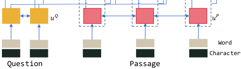
We are ready to use a BiRNN to obtain new representations  and  of all the words in the question and passage:

The notation represents the concatenation of vectors and . As implementation, it is fine to use GRU networks as BiRNN cells and setting word vector to all zeros when the word is missing from GloVe.

Question aware representation for the passage

The module after encoding computes another representation for the passage by taking into account the words inside the question sentence: a gated attention-based recurrent network is used to incorporate question information into passage representation. The difference with basic attention-based recurrent network lies in using an additional gate to determine the importance of information in the passage with respect to a particular question.

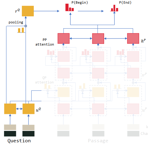
Given the question representation and the passage representation , the aim is to generate question-aware representation of the passage feeding the previous state and an attention-pooling vector into the RNN:

.

The attention-pooling vector is computed as a weighted sum

where the weights (attention scores) result from softmax

and

.

So we compute the products of matrices by vectors , take hyperbolic tangent activation tanh, multiply by a weight vector (a learned vector), then take softmax to express the “importance” of each word in the question (this is the similarity in additive attention). So we compute the product of (question representation) by the attention vector to obtain a weighted — by attention scores –average of question word vectors. is the representation of the part of the question relevant to the current word from the passage.

This is a first setup. Later S. Wang and J. Jang (2016) chose to use concatenation instead of using just (so we are considering information from the “original” input ):

.

To determine the importance of passage parts and attend the ones relevant to the question, another gate is added to the RNN input . The gate is obtained taking the product of some new weight matrix  and the concatenated vector , then using a sigmoid activation function.

.

The gate output is a vector of non-negative entries, which is then (element-wise) multiplied by the original concatenated vector

The result of this multiplication is finally passed to the RNN cell as input.

In the next section we’ll discuss the self-matching attention layer and the output layer.

Applying self-matching attention on the passage

The authors suggest to add an attention mechanism on the passage itself. This is done because the question aware passage representation has a very limited knowledge of context. Here the vector is passed as the input for the self-matching attention module. So, the question-aware passage representation is directly matched against itself. It dynamically collects evidence from the whole passage for words in passage and encodes the evidence relevant to the current passage word and its matching question information into the passage representation .

The equation for the passage representation is

where is the attention-pooling vector of the whole passage (depending on the whole passage and at time ):

Here is a weight vector, the weights matrices and are different. An additional gate as in gated attention-based recurrent networks is applied to to adaptively control the RNN input.

Output Layer: predicting the interval containing the answer to the question

Pointer networks were introduced in a paper by Vinyals et al. to address some issues from combinatorial problems where the size of the output dictionary depends on the length of the input sequence. For these kind of problems, sequence models like neural machine translation are not effective because these methods require the size of the output dictionary to be fixed a priori. In these networks the softmax probabilities arising from the attention mechanism are considered as “pointers” to input elements. For example, pointer networks works well for solving combinatorial problems like convex hull and Delaunay Triangulation.

In our context, pointer networks are used to predict the beginning and end of the answer. Given the passage representation , the attention mechanism is used as a pointer to select the start position and the end position from the passage:

Here represents the last hidden state of the answer RNN (pointer network). The initital hidden state is the output of the question pooling. The at time represent probabilities over the words in the passage, the argmax of the vector is the predicted starting point. The input of the answer RNN is the attention-pooling vector based on current predicted probability :

As initial state of the answer RNN we use the question vector . The vector is an attention–pooling vector of the question based on the parameter (as usual, the equations are those of an attention model):

There are many open source R-Net implementations, probably one of the most simple using Keras (respecting the original paper naming conventions) can be found here.